Example 0
In this introductory example, we showcase how to explore a pactus-compatible dataset. For simplicity, we built the example around a single dataset: hurrdat2 dataset. However, the same procedure can be applied to all the other datasets included in pactus.
- The example is structured as follows:
Note
You can access the script of this example.
1. Setup dependencies
Import all the dependencies:
import matplotlib.pyplot as plt
import numpy as np
from yupi.graphics import plot_2d, plot_hist

from pactus import Dataset
2. Loading Data
To load the original Hurdat2 dataset we can simply do:
ds = Dataset.hurdat2()
Then, we can inspect its content:
print(f"Loaded dataset: {ds.name}")
print(f"Total trajectories: {len(ds.trajs)}")
print(f"Different classes: {ds.classes}")
Loaded dataset: hurdat2
Total trajectories: 1903
Different classes: [1, 3, 0, 2, 4, 5]
Note
In this particular case, the classes are integers that reflect the hurrican category in the Saffir-Simpson scale. However, the classes of other datasets may be strings.
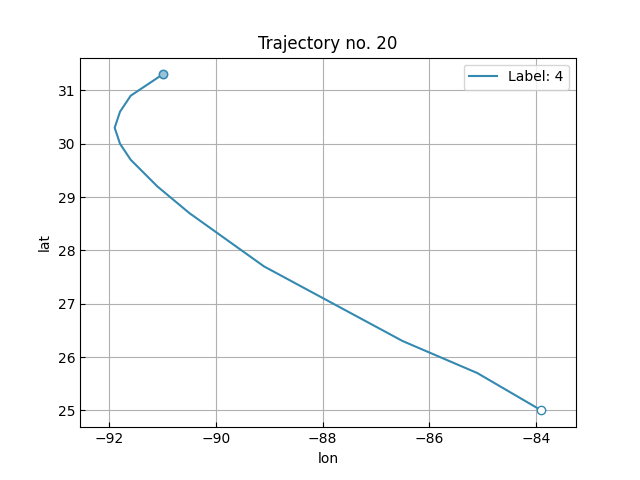
3. Inspecting a single trajectory
Here, we will pick the trajectory no. 20, and its corresponding label, from the dataset and plot it using yupi. Several operations can be performed over a trajectory. For a comprehensive guide see yupi’s documentation .
traj_idx = 20
traj, label = ds.trajs[traj_idx], ds.labels[traj_idx]
plot_2d([traj], legend=False, show=False)
plt.legend([f"Label: {label}"])
plt.title(f"Trajectory no. {traj_idx}")
plt.xlabel("lon")
plt.ylabel("lat")
plt.show()
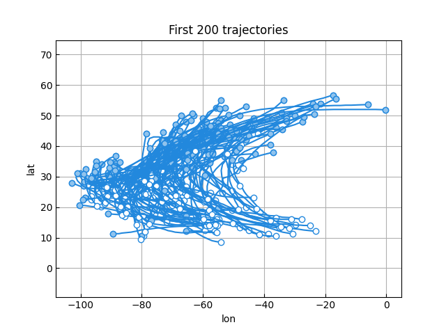
4. Inspecting a subset of the first trajectories
Similarly, we can plot a group of trajectories all together. Next, we will pick the first 200 trajectories from the dataset and plot them:
traj_count = 200
first_trajs = ds.trajs[:traj_count]
plot_2d(first_trajs, legend=False, color="#2288dd", show=False)
plt.title(f"First {traj_count} trajectories")
plt.xlabel("lon")
plt.ylabel("lat")
plt.show()
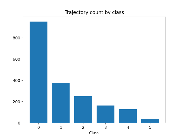
5. Inspecting the distribution of trajectories on each class
In any kind of classification, it is very useful to know the balance of a dataset among all the available classes. The following code produces a histogram with the count of trajectories on every class.
plt.bar(ds.label_counts.keys(), ds.label_counts.values())
plt.title("Trajectory count by class")
plt.xlabel("Class")
plt.show()
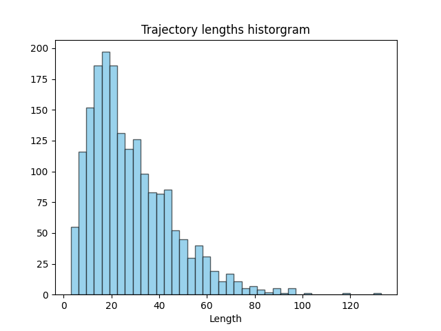
6. Inspecting the lenght distribution of the trajectories in the dataset
Another useful information to extract from a trajectory dataset is the distribution of the trajectories lenghts. The following code produces a histogram of the lenghts of every trajectory in the dataset.
lengths = np.array([len(traj) for traj in ds.trajs])
plot_hist(lengths, bins=40, show=False)
plt.title("Trajectory lengths historgram")
plt.xlabel("Length")
plt.show()